
 ">
">
Levels of income inequality depend on where you live—higher in California and parts of the Northeast and South, and lower in states in the Midwest and Mountain West. Many of the states with high levels of income inequality also have large, diverse populations and high levels of residential segregation. In 2013, only eight states had Gini indices higher than the national average—California, Connecticut, Florida, Georgia, Illinois, Louisiana, Massachusetts, and New York—but over one-third of the U.S. population (36 percent) lived in these eight states. Income inequality was highest in New York, where the top 20 percent of households controlled 54 percent of household income. States with the lowest levels of inequality included Alaska, Hawaii, Idaho, New Hampshire, Utah, and Wyoming.13
Since 1979, income inequality has increased in all 50 states and the District of Columbia. From 1979 to 1999, the increase in inequality was largest in California and several states in the Northeast, including Connecticut, Massachusetts, New Jersey, and New York. But since 1999, Illinois, Indiana, Montana, North Dakota, Vermont, and Wisconsin experienced the largest increases in inequality. The rise in Montana and North Dakota may be linked to the recent oil rush in those states, which boosted incomes but also led to a growing gap between higher-income workers in the oil industry and those in lower-paying jobs. The decline in unions, especially in Rust-Belt states, has also played a role in the rise in inequality. Up to three-fourths of the increase in inequality between white-collar and blue-collar men from 1978 to 2011 has been linked to the decrease in collective bargaining.14
Like inequality, poverty has increased in recent years, but at 14.5 percent, the rate is well below levels recorded 50 years ago when President Lyndon Johnson declared a war on poverty. Poverty rates have fluctuated over time, increasing during recessions and decreasing during periods of economic growth.
However, in many areas, poverty and inequality have increased in tandem in recent years. In the 1980s and 1990s, income inequality and poverty intersected primarily in Appalachia, the Deep South, and parts of California and the Southwest (see counties shaded orange in Figure 2). But during the past decade, poverty and inequality spread to new areas in Alabama, the Carolinas, Georgia, Michigan, and Tennessee. By 2008-2012, the majority of counties in the South (59 percent) had high levels of inequality combined with high poverty. In this analysis, counties are classified as “high poverty” if they have poverty rates greater than 15.4 percent—the average poverty rate across all of the counties and years. “High-inequality” counties are those with Gini indices greater than 0.43 (the average Gini Index across all counties and years). Nationwide, 37 percent of counties fell into this high-inequality/high-poverty category in 2008-2012, up from 31 percent in 1999 and 29 percent in 1989. In 2013, 136 million people (43 percent of the total U.S. population) lived in high inequality/high-poverty counties, more than twice the number of people who lived in high-inequality/high-poverty counties in 2000 (63 million).
In recent years, population growth has been fastest in areas with high inequality but low poverty, especially parts of the upper Midwest. Between 2010 and 2013, North Dakota was the fastest-growing state in the country, with a 7.6 percent increase in population. Among all high-inequality/low-poverty counties, the population increased by 2.7 percent from 2010 to 2013, compared with 2.2 percent growth in low-inequality/low-poverty counties, 2.0 percent growth in high-inequality/high-poverty counties, and just 0.5 percent growth in low-inequality/high-poverty areas.
These regional patterns also have a racial/ethnic component. African Americans and Latinos made up 29 percent of the U.S. population in 2013, but accounted for 41 percent of the population living in high-poverty/high-inequality counties, which are disproportionately located in the South and southwestern United States (see Figure 2). Many counties in the South are characterized by high poverty rates, high levels of residential segregation, and low levels of intergenerational mobility (economic outcomes for children relative to those of their parents). For example, in the Atlanta Metro area, only 4.5 percent of children growing up in the bottom income quintile reach the top income quintile as adults.15
Note: There are three maps in the gif.
The share of low-inequality/low-poverty counties has dropped steadily over time, from 50 percent of counties in 1989 to 44 percent of counties in 1999, to just 34 percent of counties in 2008-2012 (see Figure 3). Today, most of the remaining low-inequality/low-poverty counties are located in the upper Midwest, Mountain, Mid-Atlantic, and northeastern states.
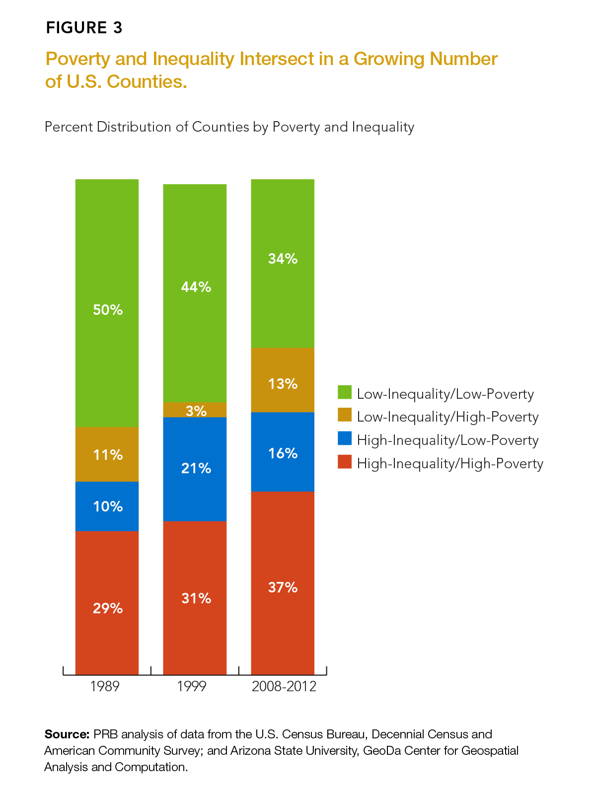
Inequality is most often discussed in the context of lower-income families but income disparities also exist in affluent communities, dividing middle-class and high-income families. The number of high-inequality/low-poverty counties peaked in 1999 during a period of rapid economic expansion and relative economic prosperity. About 21 percent of counties were classified as high-inequality/low-poverty in 1999. By 2008-2012, the share of high-inequality/low-poverty counties had dropped to 16 percent. Many of these counties are located in high-cost metropolitan areas on the East and West coasts, but there has also been a sharp increase in inequality in oil-rich North Dakota, where poverty rates remain relatively low.16
Finally, some counties have widespread poverty but a fairly narrow gap between higher-income and lower-income families. These low-inequality/high-poverty areas, almost nonexistent in 1999, made up 13 percent of counties in 2008-2012, due to job losses associated with the Great Recession, especially in parts of Maine, Michigan, Missouri, and Oregon. Also included in this group are many American Indian areas, such as Buffalo County, South Dakota, which has one of the highest poverty rates in the nation (33 percent).17
NEXT: The Generational Divide
POPULATION BULLETIN CHAPTERS
Introduction
The Backdrop: Rising Inequality
Where Poverty and Inequality Intersect
The Generational Divide
Persistent Racial/Ethnic Gaps
Women Making Progress, But Gaps Remain
Education: The Great Equalizer?
Looking Ahead
References
- U.S. Census Bureau, 2013 American Community Survey.
- Lawrence Mishel, “Unions, Inequality, and Faltering Middle-Class Wages,” in Growing Apart: A Political History of American Inequality, accessed at http://scalar.usc.edu/works/growing-apart-a-political-history-of-american-inequality/what-unions-did-labor-policy-and-american-inequality, on Aug. 30, 2014.
- Raj Chetty et al., Where Is the Land of Opportunity? The Geography of Intergenerational Mobility in the United States, accessed at http://obs.rc.fas.harvard.edu/chetty/mobility_geo.pdf, on Aug. 5, 2014.
- Mark Mather and Beth Jarosz, “U.S. Energy Boom Fuels Population Growth in Many Rural Counties” (March 2014), accessed at www.prb.org/Publications/Articles/2014/us-oil-rich-counties.aspx, on Aug. 5, 2014.
- U.S. Census Bureau, American Community Survey.