Pouring Cola

Taxes, Health-Warning Labels May Help Limit Consumption of Sugary Beverages and Improve Health

To combat obesity and diabetes, lawmakers in a number of U.S. cities have taxed sodas, sports drinks, and sweetened tea, and many are now considering health warning labels.

Growing evidence suggests that both strategies—taxes and warning labels—can reduce the purchase and consumption of sugary drinks, research supported by the Eunice Kennedy Shriver National Institute of Child Health and Human Development (NICHD) shows.

Health-Warning Labels Influence What People Buy and Consume

Even brief exposure to health warnings on sugar-sweetened beverages reduces purchases of those beverages, providing evidence that such warnings can promote healthier drink choices, a new study demonstrates.1

A team of researchers from the University of North Carolina at Chapel Hill (UNC)—including Anna Grummon, Lindsey Smith Taillie, Shelley Golden, Marissa Hall, and Noel Brewer—examined how health warnings influence what consumers actually buy in real settings. This randomized controlled trial assigned 400 consumers of sugary beverages to groups that saw either a health warning or a label that looked like a barcode.

“We worked in a convenience-store laboratory that allowed us to control whether the sugary drinks had warnings,” explains Grummon, now at Harvard University. “We are also one of the first studies to measure what consumers actually buy after seeing warnings, when they have their own money on the line.”

Participants who saw the health warning labels purchased about 22% fewer calories from sugary drinks compared with participants who saw a neutral label. The study also found that the warnings were influential across diverse groups: The effect of health warnings on beverage purchases did not differ by participants’ race/ethnicity, education, age, gender, sexual orientation, income, body weight, or health-literacy level.

According to Grummon, critics of health warning labels argue that consumers won’t notice or pay attention to the warnings. However, three-quarters of the participants in this study reported noticing the health warnings, and most of those participants also reported that they read and looked closely at the labels.

In another study, Grummon and Hall synthesized the findings of 23 studies and found that health warnings labels not only reduced purchases of sugary drinks but also caused stronger emotional responses, increased perceptions that sugary drinks contribute to disease, and reduced intentions to purchase or consume sugary drinks.2 All these responses are key indicators when it comes to long-term behavior change, they note.

“Our findings suggest that sugary drink warnings help consumers better understand products’ healthfulness and encourage them to make healthier choices about what drinks to buy,” says Grummon.

In a related mathematical simulation, UNC researchers show that a national policy requiring health labels on sugar-sweetened beverages could reduce obesity prevalence by about 3.1 percentage points over five years, if sustained.3

“While three percentage points might sound modest, on a national scale it equates to more than five million fewer people with obesity,” says Grummon. “Warnings are a highly scalable strategy for helping consumers make healthier choices. These findings suggest that warnings are also promising for addressing obesity in the U.S.”

Improved Child Health Projected in Wake of Mexico’s Soda Tax

The Mexican government enacted the first national tax on sugar-sweetened beverages after a 2012 study indicated that more than 70% of the country’s population was overweight or obese, and that in excess of 70% of the added sugar calories in the Mexican diet were coming from sugary drinks.

In the two-year period spanning 2014 to 2015, a research team that included Barry M. Popkin and Shu Wen Ng of UNC found that:

  • The one-peso-per-liter excise tax on sugar-sweetened beverages in Mexico resulted in a 6% reduction in purchases of taxed beverages during the first year and continued to decline, with a 10% decrease in purchases in the second year.
  • During the same study period, purchases of untaxed beverages such as bottled water increased 2.1%.
  • Residents of households with lower socioeconomic levels, for whom health care costs are most burdensome, reduced their purchases of sweetened beverages the most.4

The findings run counter to initial reports from the sugar-sweetened soda industry, which said that the purchases of sugary drinks actually went up after the initial tax year. However, the researchers found those reports did not account for numerous significant factors, including inflation and shifts in population.

In addition, a new analysis co-authored by Popkin estimates that Mexico’s sugar-sweetened beverage tax could result in meaningful weight control and life-long health benefits for the country’s children and adolescents, particularly those who had been high consumers of the beverages before the tax.5 Childhood obesity is a strong predictor for obesity later in life, which can also lead to chronic illnesses such as diabetes, hypertension, and heart disease, the researchers emphasize.

To estimate the one-year effect of the tax on the body weight of children ages 5 to 17, by taking into account patterns of childhood growth and obesity in Mexico and assuming that the known reductions in sugar-sweetened beverage purchases would reflect changes in consumption.

Findings show that one year after the implementation of the current tax, children and adolescents should experience an average reduction in body weight of 0.26 and 0.61 kg (one kilogram equals about 2.2 pounds). For those who had been high consumers of sugary drinks, the team estimates the positive impact on body weight would be even greater, with an average body weight reduction of 0.50 kg for children and 0.87 kg for adolescents. Sustained over several years, such weight loss could mean some children and adolescents would not longer be considered obsese.

“Taxation represents one of the most effective ways to reduce consumption of unhealthy sugar-sweetened beverages, which can make a meaningful impact on future excessive weight gain and significantly reduce the long-term risks of becoming obese,” says Popkin. “If the taxation revenue is used to support child and adolescent healthy eating, then the benefits of such taxes are enhanced.”

Public Support Is Key to Policies Limiting Sugary Beverages

For taxes on sugary beverages to become a widely used strategy for improving public health, public support and acceptance are key.

Public opinion on the policies’ unintended consequences may affect attitudes toward the policy, argue Melissa Knox, Jessica Jones-Smith, and Vanessa Oddo of the University of Washington, who analyzed perceptions of the effects of Seattle’s 2017 sugary beverage tax.6

“We find that a majority of participants (59%) support the sugary beverage tax in Seattle and correspondingly, most people believed that the tax will positively impact health, and will not negatively affect general and personal economics in Seattle,” they report. “However, lower-income, versus higher-income, respondents were more concerned about the possible negative economic consequences of the tax,” such as job loss or increased financial costs for their family and friends.

A related study shows that attitudes toward sugary beverage taxes may be difficult to accurately estimate in phone surveys.7 Phone respondents (but not web respondents) under-report their sugary beverage consumption by about 25% and over-report positive attitudes toward the tax by about 11%, the researchers determined. These differing results likely reflect respondents’ answering interviewers’ questions in ways they believe are more socially desirable or acceptable rather than choosing responses that reflect their true thoughts or feelings, a tendency known as social desirability bias.

The researchers offer advice to lawmakers implementing soda taxes.

  • Policymakers “should be wary of solely relying on self-reported measures of intake when evaluating the effectiveness of these policies,” they write, noting that consumers may consume more sweetened beverages than they report.
  • Lawmakers should strengthen “their public messaging regarding the health and economic benefits of sweetened beverage taxes, even if they believe that attitudes are generally positive. Without a pro-tax messaging campaign that informs the public about the positive health and economic effects of these taxes, the taxes may eventually lose public support.”

The researchers point out that “recent successful efforts to block U.S. municipalities from enacting future beverage taxes by banning the taxes at the state level have relied heavily on informational campaigns that focused on the negative economic effects of the taxes. These campaigns, often funded by the beverage industry, may ultimately shift social norms in the direction of more favorable attitudes toward sweetened beverages, with unpredictable effects on public health.”


This article was produced under a grant from the Eunice Kennedy Shriver National Institute of Child Health and Human Development (NICHD). The Communications and Marketing team at the Gillings School of Global Public Health at the University of North Carolina at Chapel Hill contributed to this article. The work of researchers from the following NICHD-funded Population Dynamics Research Centers was highlighted: University of North Carolina at Chapel Hill (P2CHD050924) and University of Washington (5P2CHD042828-18).


References

  1. Anna H. Grummon et al., “Sugar-Sweetened Beverage Health Warnings and Purchases: A Randomized Controlled Trial,” American Journal of Preventive Medicine 57, no. 5 (2019): 601-10.
  2. Anna H. Grummon and Marissa G. Hall, “Sugary Drink Warnings: A Meta-Analysis of Experimental Studies,” PLOS Medicine (2020), https://doi.org/10.1371/journal.pmed.1003120.
  3. Anna H. Grummon et al., “Health Warnings on Sugar-Sweetened Beverages: Simulation of Impacts on Diet and Obesity Among U.S. Adults,” American Journal of Preventive Medicine 57, no. 6 (2019): 765-74.
  4. M. Arantxa-Colchero et al., “In Mexico, Evidence of Sustained Consumer Response Two Years After Implementing a Sugar-Sweetened Beverage Tax,” Health Affairs 36, no. 3 (2017): https://doi.org/10.1377/hlthaff.2016.1231
  5. Rossana Torres-Álvarez et al., “Body Weight Impact of the Sugar-Sweetened Beverages Tax in Mexican Children: A Modeling Study,” Pediatric Obesity 15, no. 8 (2020): e12636, https://doi.org/10.1111/ijpo.12636.
  6. Vanessa M. Oddo et al., “Perceptions of the Possible Health and Economic Impacts of Seattle’s Sugary Beverage Tax,” BMC Public Health 19 (2019): 910.
  7. Melissa A. Knox et al., “Is the Public Sweet on Sugary Beverages? Social Desirability Bias and Sweetened Beverage Taxes,” Economics & Human Biology 38 (2020): 100886.
New_1120f-cohabiting

Cohabiting Couples in the United States Are Staying Together Longer but Fewer Are Marrying

More unmarried couples today are living together, and doing so for longer than in the past, but fewer of these relationships lead to marriage, new research finds. This change may in part reflect shifting attitudes toward cohabitation, and it results in more separations and re-partnering during young adulthood.

Most young women today will live with a romantic partner at least once, compared with just one-third of young women in the late 1980s.1 During that decade, most cohabiting relationships were short-lived and frequently led to marriage.

The new research, conducted by graduate students and faculty at the Center for Family and Demographic Research at Bowling Green State University, examined how cohabitation and marriage patterns have changed for young women over the past four decades. Their research was supported by the Eunice Kennedy Shriver National Institute of Child Health and Human Development (NICHD).

In their study, Esther Lamidi, now at the University of Colorado Colorado Springs, and colleagues Wendy Manning and Susan Brown at Bowling Green, drew on data from the National Survey of Family Growth (NSFG) to compare women ages 15 to 39 who lived with a first romantic partner in 1983-1988 and in 2006-2013.They examined changes in whether couples who lived together had married or split up within five years.

They found that while cohabiting relationships are still relatively short-lived, couples today are cohabiting longer—increasing from about 12 months in the 1983-1988 cohabitation cohort to 18 months in the later cohort—and that this longer duration is linked to couples delaying or forgoing marriage altogether. After five years, similar shares of women in both cohorts were still living with their partner, but the distribution of those still cohabiting as compared to those who had married had shifted. Among the early cohort, 23% of women were still cohabiting five years later, and 42% had married their partner. These shares were reversed among the later cohort—43% were still cohabiting and only 22% had married.

Women With Less Education Experience More Changes in Cohabitation

Over the past five decades, changes in family behaviors such as declining rates of marriage have been more pronounced among women with less education compared with women who have more education. Lamidi and her colleagues confirmed this divergence—similar to what’s been observed in other family behaviors and frequently termed “diverging destinies”—when they examined patterns of cohabitation across different sociodemographic groups.

Their analysis found that the more recent cohort was much less likely to marry their cohabiting partner, and while this pattern was observed across all sociodemographic groups, it occurred more frequently among women with less education.

After accounting for women’s educational attainment, their results show that between the two cohorts only women with less than a college education experienced a decline in marrying their cohabiting partner. In addition, women having one or more children while cohabiting—an occurrence more common among women with less education—delayed or inhibited marriage more for the later cohort than the earlier cohort, they found.

Cohabitation Changes Reveal a Widening Social Class Divide

Sociodemographic characteristics are associated with the pathways out of cohabitation—break ups or marriages—and changes among the cohabiting population’s characteristics can be reflected in changes in cohabitation outcomes. Yet while the researchers noted that the cohabiting population grew in size, became more racially and ethnically diverse and more highly educated, and had more births while living together, they found these compositional changes had little impact on the changes in cohabitation outcomes across the two cohorts.

What does this finding mean? The researchers conclude that the limited impact of population composition changes on cohabitation outcomes, combined with the decline in marrying a cohabiting partner among women with less education, suggests that the social class divide in the American family appears to be widening.

Their findings also “diminish the traditional view of cohabitation as a prelude to marriage” for women with less education and show, particularly for this population, that “cohabitation is increasingly serving a role similar to that of traditional marriage in offering a viable context for childbearing and child-rearing.”

Young Women Today Are Increasingly Likely to Experience a Breakup

Although cohabiting relationships may be lasting longer, they remain relatively unstable. Kasey Eickmeyer, now at the Center for Policing Equity, reports, “Millennials experienced more relationship instability during young adulthood than earlier birth cohorts of women.” She found that cohabitation experience accounted for this instability.

Eickmeyer asked whether young women see their intimate live-in relationships (either marriage or cohabitation) end more frequently today than earlier generations.3 She analyzed data from multiple cycles of the NSFG to examine women’s experience of ending marriages and cohabiting relationships when they were ages 18 to 25 across several five-year birth cohorts from 1960 to 1985.

She found that among women who had ever married or cohabited, the share breaking up with a live-in partner increased from 31% among women born between 1960 and 1964 to 44% among women born in 1985 to 1989.

Cohabitation explains this increasing likelihood of experiencing a breakup. Compared to women in the 1985-1989 birth cohort, women in the earlier birth cohorts from 1960-1964 through 1975-1979 were significantly less likely to have one or more live-in partnerships end. Once Eickmeyer accounted for women’s cohabitation experience, she found that young women’s increased likelihood of having an intimate partnership end is because union formation during young adulthood shifted from marriage—a relatively stable union—to cohabitation, a relatively unstable union.

More Breakups and Re-Partnering in Young Adulthood Suggest Changing Attitudes About Cohabitation

As more young women enter into and end cohabiting relationships, they have more opportunities to live with multiple partners in a pattern of serial cohabitation. The growing practice of serial cohabitation reflects in part changing attitudes about couples living together without marriage.

Eickmeyer and Wendy Manning wanted to know whether contemporary young adult women who had ever cohabited are more likely to re-partner than prior cohorts of young women.4 Using data from the 2002 and 2006-2013 NSFG, they compared the cohabitation experience of young women ages 16 to 28 across five-year birth cohorts beginning in 1960 through 1980 to examine trends in serial cohabitation.

They found that early Millennial women (born 1980-1984) were 53% more likely to live with more than one romantic partner during young adulthood compared with the late Baby Boomers (born 1960-1964), even after taking into account sociodemographic characteristics such as race and ethnicity and educational level, and relationship characteristics such as their age when their first cohabiting relationship ended and whether they had children.

Not only were early Millennial women more likely to live with more than one partner without marriage, they also formed subsequent cohabiting relationships more quickly than the late Baby Boomers—dropping from nearly four years between live-in relationships to just over two years.

The characteristics most strongly associated with serial cohabitation—such as identifying as non-Hispanic white, having less than a college education, and growing up with a single parent—remained stable across birth cohorts, Eickmeyer and Manning found. And, much like the cohabiting population, the composition of women who had previously lived with a partner changed across cohorts, but this shift does not explain the increase in serial cohabitation.

The researchers conclude that the increase stems from more young adults cohabiting, the continued instability of cohabiting relationships, the increasing length of time between first cohabitation and first marriage, and the growing acceptance of cohabitation during young adulthood.

Their findings highlight the instability in many contemporary young adults’ lives and the increasing role cohabitation plays in relationship churning. Although multiple live-in romantic relationships could have negative consequences for young adults’ well-being (and any children they may have), Eickmeyer and Manning suggest “that young adult relationships may be evolving, and young women may be learning to end coresidential relationships that are not working.”


This article was produced under a grant from the Eunice Kennedy Shriver National Institute of Child Health and Human Development (NICHD). The work of researchers from the NICHD-funded population dynamics research center at Bowling Green State University (P2CHD050959) was highlighted in this article.


References

  1. Paul Hemez and Wendy D. Manning, Twenty-Five Years of Change in Cohabitation in the U.S., 1987-2013, National Center for Family and Marriage Research Family Profiles, No. FP-17-02 (2017), http://www.bgsu.edu/ncfmr/resources/data/family-profiles/hemez-manning-25-years-change-cohabitation-fp-17-02.html
  2. Esther O. Lamidi, Wendy D. Manning, and Susan L. Brown, “Change in the Stability of First Premarital Cohabitation Among Women in the United States, 1983-2013,” Demography, 56 (2019): 427-50.
  3. Kasey J. Eickmeyer, “Cohort Trends in Union Dissolution During Young Adulthood,” Journal of Marriage and Family 81 (2019): 760-70.
  4. Kasey J. Eickmeyer and Wendy D. Manning, “Serial Cohabitation in Young Adulthood: Baby Boomers to Millennials,” Journal of Marriage and Family 80 (2018): 826-40.
New_0820f-incarceration

When a Parent Is Incarcerated, Partners and Children Also Pay a Price

“We live in a country where we have huge numbers of children exposed to parental incarceration. When we talk about the need to reform the criminal justice and mass incarceration systems, we also need to talk about the unintended victims of the current system,” says Christine Leibbrand of the University of Washington. “Incarceration exposes families to poverty and disadvantage, and the system can self-perpetuate inequality.”

About 3.5% of U.S. children under age 18—or one child in every classroom of about 29 students—had a parent behind bars in 2015, mainly their fathers.1

Black children were more than five times more likely than white children to be separated from a parent by incarceration, report sociologists Bryan Sykes of University of California, Irvine and Becky Pettit of University of Texas at Austin. These patterns reflect a system that disproportionately imprisons disadvantaged and minority men, they argue.

A growing body of research documents the toll U.S. incarceration takes on the families of those imprisoned, widening disparities and exacerbating existing disadvantages. New research supported by the Eunice Kennedy Shriver National Institute of Child Health and Human Development provides further evidence on the wide-ranging ways a parent’s incarceration shapes the lives and life chances of their partners and children, from the neighborhoods where they live to the levels of adversity their children experience.

Children of Incarcerated Fathers Are More Likely to Live in High-Poverty Neighborhoods and Move More Often

Children whose fathers were incarcerated move more frequently and live in neighborhoods that are more socioeconomically disadvantaged than their peers whose fathers have never been in prison, find Leibbrand and Erin Carll of the University of Washington, Angela Bruns of the University of Michigan now at Gonzaga University, and Hedwig Lee of Washington University in St. Louis.2

Using data from the national Fragile Families and Child Wellbeing Study—research following thousands of families in 20 large U.S. cities since 1998—the team examined the neighborhoods of children whose fathers were in prison or recently released. Families with a father currently or recently in prison tend to live in neighborhoods with higher percentages of residents who are single mothers, receive public assistance, lack a high school diploma, and live below the poverty line, they show.

The financial hardship families with imprisoned members face, researchers say, perpetuates what they call “downward mobility.” A father in prison is one less wage earner at home or paying child support. Families with limited income have fewer choices of where to live, they may move often, and the neighborhoods they end up in may be marked by lower quality schools, greater unemployment, and higher rates of crime and violence, Leibbrand and her colleagues report.

“When we think about where people live or move to, we think of people weighing the pros and cons of different places. That’s far too simple. Many families may be forced to move because of eviction or budget constraints, for example, and these forced moves are often to worse neighborhoods where families have little choice of where they would like to live,” says Leibbrand.

Mothers With a Partner in Prison Are More Likely to Hold Multiple Jobs

Mothers with incarcerated partners are more likely to work multiple jobs than women in otherwise similar circumstances, finds Bruns in another study.3

Partner incarceration is linked to additional employment—a third shift—on top of the paid work and caregiving women already do, she finds, based on analysis of Fragile Families and Child Wellbeing Study data.

An additional job may cover basic expenses but also compounds the burden that women with incarcerated partners already shoulder, she points out.

“Staying in touch and supporting an inmate—responding to his requests for food, clothing and books, preparing packages to the correctional institution’s specifications, coordinating family member visits, and keeping up with legal cases and appeals—can feel like a second job in and of itself,” explains Bruns.

Mothers with partners who are incarcerated usually have sole responsibility for children who may be “struggling with the absence of their fathers,” according to Bruns. Holding multiple jobs is also a known stressor that could raise mothers’ risk of stress-related health conditions.

Low-skilled women are often stuck in low-wage, dead-end jobs that can barely pay the bills, she asserts.

“Balancing multiple work roles in addition to family member incarceration may keep women from going to school or participating in other activities that improve their socioeconomic standing over the long-term,” writes Bruns.

Youth With a Parent in Prison Face More Trauma and Adversity

Youth ages 11 to 17 who experience the incarceration of a parent are more likely to have behavioral problems or mental health issues than their counterparts whose parents have never been jailed, Samantha J. Boch, Barbara L. Warren, and Jodi L. Ford of Ohio State University show.4

The team finds that household poverty plays a role, as does the number of traumatic events the young person has experienced, including homelessness, eviction, foster care, and serious injury or death in the family. Overall, they find that youth who deal with the incarceration of a parent experience three times as many adverse childhood experiences (ACEs) as their unaffected peers.

The researchers base their analysis on interviews with more than 600 parents or other caregivers participating in the Adolescent Development in Context study, a representative sample of Columbus, Ohio, and its surrounding suburbs.

The behavioral problems and mental health issues exhibited more frequently in children who experience a parent’s incarceration include poor attention, excessive anxiety, and externalizing behaviors such as rule breaking, temper outbursts, and property destruction, the analysis finds.

The researchers examined a wide-ranging set of 30 ACEs that includes aspects of financial distress and household churning or instability such as changes in household composition (for example, when a parent or parent’s new partner leaves or joins the household or when a child goes to live with grandparents) and residential moves.

“Well-documented research investigating the cumulative effect of ACEs indicates that youth exposed to parental incarceration may have a much greater likelihood for engaging in maladaptive coping behaviors (such as cigarette, alcohol, and illicit drug use, or violent delinquent behaviors) and experiencing depression, anxiety and post-traumatic stress disorder across the lifespan,” the researchers report.

They argue that mental health providers should view a parent’s incarceration as an important consideration of the child’s and family’s well-being that warrants continued observation, support, and follow-up. More research is needed to determine the best ways to screen and identify these youths using non-stigmatizing approaches that build on their strengths, they suggest. 

A Parent’s Incarceration Can Shape a Child’s Identity and Influence Anti-Social Behavior

Among young adults with an incarcerated parent, those who had a high need for parental approval were more likely to identify themselves as a troublemaker or partier during young adulthood than those who were emotionally independent, a recent study finds.5

Self-identities influence behavior, including criminal activity, making understanding the precursors of self-identity important to interventions designed to improve the life prospects of children with incarcerated parents, according to the researchers Jessica G. Finkeldey of the State University of New York at Fredonia, and Monica A. Longmore, Peggy C. Giordano, and Wendy D. Manning of Bowling Green State University.

The team examined publicly available incarceration records and analyzed data from the Toledo Adolescent Relationships Study, a regional survey of more than 900 men and women ages 18 to 28 interviewed five times between 2001 and 2011.

Developing “high emotional independence, or values, beliefs, and identities in contrast to and separate from an incarcerated parent,” may set young adults on a path shaped by different choices than those made by their incarcerated parent, the researchers suggest.

“It is possible that exposing children of incarcerated parents to positive role models and mentors, such as through mentorship programs, might help to reduce the transmission of antisocial identities and behaviors and should be investigated,” says Finkeldey.


This article was produced under a grant from the Eunice Kennedy Shriver National Institute of Child Health and Human Development (NICHD). The work of researchers from the following NICHD-funded population dynamics research centers was highlighted in this article: University of Washington, University of Michigan, Ohio State University, Bowling Green State University, and University of Texas at Austin.


References

  1. Bryan L. Sykes and Becky Pettit, “Measuring the Exposure of Parents and Children to Incarceration,” in Handbook on Children with Incarcerated Parents, ed. J. Mark Eddy and J. Poehlmann-Tynan, (Geneva: Springer, 2019): 11-23.
  2. Christine Leibbrand et al. “Barring Progress: The Influence of Parental Incarceration on Families’ Neighborhood Attainment,” Social Science Research 84 (2019): 102321
  3. Angela Bruns, “The Third Shift: Multiple Job Holding and the Incarceration of Women’s Partners,” Social Science Research 80 (2019): 202-15.
  4. Samantha J. Boch, Barbara L. Warren, and Jodi L. Ford, “Attention, Externalizing, and Internalizing Problems of Youth Exposed to Parental Incarceration,” Issues in Mental Health Nursing 40, no. 6 (2019): 466-75.
  5. Jessica G. Finkeldey et al. “Identifying as a Troublemaker/Partier: The Influence of Parental Incarceration and Emotional Independence,” Journal of Child and Family Studies 29, no. 3 (2020): 802-16.
new_0720f-young-adult-struggle

Life on Hold: How the Coronavirus Is Affecting Young People’s Major Life Decisions

The past two decades have been tumultuous for the United States. During the first 20 years of the 21st century, the nation experienced a major terrorist attack, a housing market meltdown, a severe economic recession, a significant downturn in the stock market, and a pandemic that led to the highest unemployment rate since the Great Depression.

The coronavirus and the disease it causes, COVID-19, are affecting all Americans. Older people are most at risk of severe health issues related to the virus, but young adults—ages 25 to 34—may be most vulnerable to its long-term social and economic impacts. Those in their early 30s reached young adulthood during the Great Recession of 2007 to 2009 and experienced one of the most challenging job markets in U.S. history. Now those in their mid-20s are entering prime marriage and family formation years just as the coronavirus pandemic is causing extensive economic and social disruptions.

Even before the crisis hit, more young Americans had been postponing key life events that often mark the transition to adulthood. Fewer young adults in their 20s and 30s are getting married, having children, living independently from their parents, buying homes, and achieving financial independence. Nearly one in five young adults ages 25 to 29 are disconnected from work and school. A growing share of young adults carry high levels of student loan and credit card debt that may cause them to postpone marriage and family formation.1 The pandemic will likely amplify these trends.

The statistics are grim. More than 40 million workers filed for unemployment benefits in the spring of 2020. Millions of young adults work in restaurants and other service-sector jobs that have been heavily affected by stay-at-home orders and social distancing measures. The pandemic is also exacerbating the wide economic disparities between whites and other groups—especially Blacks and Latinos—who are more likely to be working in low-wage jobs with few benefits.

The current health and economic crisis is unprecedented, making it difficult to predict the impact on patterns of marriage, childbearing, homeownership, and living arrangements of young adults in the coming months and years. But we can look back at recent trends for clues.

The Coronavirus Could Prompt Many to Postpone Marriage

While the Great Recession may have forced some young adults to postpone key life transitions—such as finding a full-time job or buying a home—the decline in the proportion who are married is a longer-term trend that predates the economic downturn. It’s hard to gauge whether the decline in marriage during the recession was due to economic factors or just a continuation of previous trends.

The coronavirus may be different. In the short term, it will force millions of young adults to consider postponing marriage until social distancing restrictions are lifted. Longer-term effects on marriage are more difficult to predict.

On the one hand, some young adults—particularly those with less education and lower incomes—may decide to postpone marriage until the economy recovers, which could take years. The “economic prerequisites for entering marriage are higher today than they were for previous generations.”Meeting those requirements—finding a job, achieving some financial independence, accumulating some savings, and perhaps buying a home—may be harder than ever in the current environment, especially for lower-income workers without college degrees.3

The decline in the proportion married among young adults with lower levels of education accelerated during the Great Recession and has continued over the past decade (see Figure 1). The proportion of college graduates who are married has also declined but at a slower pace, which has led to a growing marriage gap between those at different education levels.4

FIGURE 1. Share of Young Americans Ages 25 to 34 Who Are Married (Spouse Present), by Educational Attainment, 2000-2025

Note: Projections are calculated by applying the average rate of change during the Great Recession and its aftermath to future years.
Source: IPUMS-Current Population Survey, University of Minnesota, www.ipums.org.

Between 2000 and 2019, the proportion of young adults without bachelor’s degrees who were married dropped 16 percentage points to 37%. But for college graduates, the proportion dropped just 10 percentage points to 46%. The fallout from the coronavirus could exacerbate the marriage gap for people at opposite ends of the education ladder.

If patterns since the Great Recession continue, about one-third (32%) of young adults without bachelor’s degrees may be married by 2025, compared with 42% of young adult college graduates.

On the other hand, marriage provides an opportunity to pool resources and offers tax and health coverage benefits that may be attractive to some young adults who were on the fence about tying the knot.5 A key factor contributing to the recent decline in marriage rates, especially for less-educated groups, has been the rise in women’s earnings relative to men.6 As women’s wages have increased, fewer women have relied on a spouse or partner to provide a paycheck. However, the current economic crisis may disproportionately affect women, who are more likely to be employed in service-sector jobs. A rise in “marriageable men” relative to women could potentially lead to an increase in the proportion of young adults who marry in the coming years.7

Cohabitation Expected to Increase Among Young Adults

As marriage rates among young adults have declined in recent years, cohabitation rates have increased, either as a precursor to or substitute for marriage.

The share of young women ages 25 to 34 living with a partner more than doubled between 2000 and 2019, from 7% to 22% (see Figure 2). For men, cohabiting increased from 8% to 19% during the same period. The share of young adults who have ever cohabited is much higher and increasing. In 1995, nearly half (49%) of women ages 25 to 29 had ever cohabited, but that share rose to 73% in 2011 to 2013.8

FIGURE 2. Share of Young American Men and Women Ages 25 to 34 Living With a Cohabiting Partner, 2000-2025

Notes: A change in methods used to identify cohabiting couples accounts for part of the increase in cohabitation in 2007. Projections are calculated by applying the average rate of change during the Great Recession and its aftermath to future years.
Source: U.S. Census Bureau, Current Population Survey.

Cohabiting relationships in the United States tend to be short, with most couples breaking up or getting married within a few years. Serial cohabitation—a pattern of multiple, nonmarital cohabiting relationships—is also increasingly common, especially among couples with lower levels of education.9

Will more young adults choose to live together because of the coronavirus pandemic’s impact on the economy? In the short term, anecdotal evidence suggests that social distancing measures have “fast-tracked many relationships” among couples forced to choose between living separately indefinitely and moving in together.

Other couples may decide to postpone cohabiting until economic prospects improve. Population Reference Bureau projections indicate that the share of young adult women and men who are cohabiting could rise to 22% and 19%, respectively, by 2025.

U.S. Fertility Rate Is at a Record Low and Could Fall Even Further

Some have speculated that the coronavirus pandemic will lead to a baby boom, with so many couples stuck at home due to social distancing requirements. But the research suggests otherwise.

The U.S. total fertility rate (TFR) has declined during previous economic downturns, and the current economic crisis will likely have a similar impact on births. The TFR fell to low levels during the Great Depression in the 1930s, amid the 1970s oil shock, and with the Great Recession in 2007. Fertility in the United States recently dropped to the lowest level in recorded history, with women having an average of 1.7 births in their lifetime.

The timing of childbearing has also changed. Delays in marriage have in turn resulted in delays in first births. In 2018, the average age of first-time mothers was 27, up from 25 in 2000. By 2016—for the first time in U.S. history—the birth rate among women ages 30 to 34 (103 births per 1,000 women) exceeded that of women ages 25 to 29 (102 births per 1,000 women) (see Figure 3).

FIGURE 3. U.S. Births per 1,000 Women, by Age Group, 2000-2025

Note: Projections are calculated by applying the average rate of change during the Great Recession and its aftermath to future years.
Source: U.S. Centers for Disease Control and Prevention, National Center for Health Statistics.

The economic impact of the coronavirus may cause more young adults to postpone births, leading to further declines in birth rates, especially among women under age 30.

States like Nevada, which relies heavily on tourism, may see bigger declines in fertility than states with more diversified economies. Fertility declines during the Great Recession were greatest in states most impacted by the economic downturn.10

Homeownership Among Young Adults Has Dropped Sharply Since 2007

Searching for a home right now is challenging because of social distancing guidelines, but the longer-term effects of the coronavirus on the housing market could linger for years. Millions of Americans who have been temporarily or permanently laid off may lose income and have to dip into their savings, decreasing their ability to secure a loan or make a down payment on a house. Many existing homeowners may need to sell their homes to help pay the bills.

The homeownership rate among young adults declined with the onset of the subprime mortgage crisis in 2007 and has continued to drop (see Figure 4). Between 2007 and 2019, householders ages 65 and older experienced a modest decline in homeownership (1 percentage point), whereas rates dropped sharply for householders ages 25 to 34 (8 percentage points) and 35 to 64 (9 percentage points).

FIGURE 4. U.S. Homeownership Rates by Age of Householder, 2000-2025

Note: Projections are calculated by applying the average rate of change during the Great Recession and its aftermath to future years.
Source: IPUMS-Current Population Survey, University of Minnesota, www.ipums.org.

Historically, young adults (ages 25 to 34) have had lower homeownership rates than adults ages 65 and older, and the gap between these two groups has increased 4 percentage points from 2000 to 2019. By 2025, this gap could grow even wider, according to PRB’s projections. By 2025, just 34% of householders ages 25 to 34 may be homeowners, compared with 80% of householders ages 65 and older.

Although this trend may suggest a change in housing preferences, more than two-thirds of renters report that they would buy a home if they had the financial resources to do so.11 The decline in homeownership has also been linked to lower rates of marriage and family formation among young adults.12 The share of young men and women ages 25 to 34 living with a spouse dropped from 50% and 57%, respectively, in 2000 to 36% and 45%, respectively, in 2019.13

Wide gaps in homeownership rates also persist across different racial and ethnic groups. During the housing market crisis, owning a home became a liability for many Americans but especially for African Americans and Latinos, who were more likely to have high-cost or subprime mortgages. Black and Latino workers were disproportionately low income prior to the coronavirus pandemic, and the current economic crisis could further impact the ability of Black and Latino young adults to qualify for loans or make their mortgage payments in the coming months.

More Young Adults Are Expected to Live With Parents

Declines in marriage have been accompanied by an increase in young adults—especially men—returning to or remaining in their parents’ homes, and the coronavirus pandemic will likely intensify this trend.

Between 2000 and 2019, the share of young men ages 25 to 34 living with their parents rose from 12% to 22% (see Figure 5). The share of young women living with their parents increased from 8% to 15% during the same period. For both men and women, the proportion who were doubling up with their parents in 2019 was at or near the highest levels since the U.S. Census Bureau first started tracking the measure in 1960.

FIGURE 5. Share of Young American Men and Women Ages 25 to 34 Living With Their Parents, 2000-2025

Note: Projections are calculated by applying the average rate of change during the Great Recession and its aftermath to future years.
Source: U.S. Census Bureau, Current Population Survey.

The rising number of young adults living with their parents, often disconnected from work and school, may lead to further declines in marriage, family formation, and childbearing. About 22% of young men and 15% of young women are projected to be living in their parents’ homes by 2025.

The Effects of the Coronavirus Could Last for Decades

The coronavirus pandemic could be the most significant event that will occur in our lifetime and will likely have long-lasting effects on marriage, family formation, poverty, and health in the United States. Some have pointed to the positive effect of the pandemic on bringing families together, but researchers have also shown that entering the job market during a period of economic turmoil can have long-term, negative consequences for young adults. In midlife, they earn less (while working more), are less likely to be married, are more likely to be childless, and are more likely to die prematurely compared with young adults who enter the workforce during a healthier economy.14 Young adults who entered the job market during the Great Recession are still feeling the impact.

Blacks and Latinos have been disproportionately affected by layoffs due to the pandemic, and the negative effects on Black and Latino young adults will likely linger for years—exacerbating long-standing social, economic, and health inequalities between whites and other racial/ethnic groups.

Right now, life is on hold for millions of Americans. We cannot predict the long-term effects of this crisis, but it’s likely that young adults will be severely impacted by the economic fallout. Making sure these young adults have the resources they need to cover their basic needs and access educational, employment, and training opportunities—both during and after the pandemic—will be an ongoing challenge for federal, state, and local policymakers for many years.

Empty college dorm room

Coronavirus and the 2020 Census: Where Should College Students Be Counted?

UPDATE: 2020 Census operations are changing in response to the coronavirus pandemic. The U.S. Census Bureau announced on June 18, 2020, that it is reaching out to colleges and universities with significant off-campus student populations to help ensure they are counted in the right place in the 2020 Census. College and university presidents have been asked to provide roster and basic demographic information already provided to the university for off-campus students. This information allows the Census Bureau to count the students where they would have been staying on April 1, 2020, even if they went home early due to a school closure or shift to distance learning. It can also be used to remove duplicate responses to the census or to count students (if there is no other record of the same individuals in another location). Census Bureau staff began calling school officials on June 16.


Just as the 2020 Census is getting underway, many colleges and universities across the country are closing their campuses and moving classes online in response to concerns about the coronavirus and the disease it causes, COVID-19.

Where should college students be counted in the 2020 Census? Census Bureau officials say students living away from home should be counted at their on-campus or off-campus college address, even if coronavirus has temporarily sent them to stay with their parents or elsewhere.

Most of the students moving out of their on-campus dorms and residence halls won’t return until after Census Day, which is April 1, 2020. While some students living off-campus may choose not to leave, many are returning to their prior residence (such as a family home) during these campus closures.

According to the Census Bureau’s Official Residence Criteria for the 2020 Census, college students will be counted at their “usual residence” on April 1, 2020 or where they live and sleep “most of the time.”

This means that college students will be counted at their college address (either on- or off-campus), even if they are staying at their parents’ or guardians’ home on Census Day while on break, vacation, or due to COVID-19 closures. An accurate count of students—temporarily displaced due to the pandemic—is critical for towns and cities that are home to large numbers of college students. Student populations factor into disaster planning and emergency response, public health analysis and planning, infrastructure planning, government funding allocations, and many more policy and program decisions.

How Do Colleges Count Students Living On-Campus?

Every college or university is responsible for providing the Census Bureau with a total count of students living in university-run housing, which may include fraternities and sororities.

Many schools transmit this information electronically using their housing administrative records. Some, however, opt to distribute Individual Census Questionnaires to students, who complete them and return them to the school, which passes the completed forms to a Census Bureau enumerator. With many campuses closed due to COVID-19, the Census Bureau will be reaching out to those schools and inviting them to switch to the electronic option.

Either way, it is the responsibility of the college or university to gather the necessary information and provide it to the Census Bureau. Students living in on-campus or in university-run housing should not complete the census online or by telephone.

If a student living on-campus or in university-run housing is unsure about what to do regarding the 2020 Census, they should contact their college’s housing administration office or the Census Bureau.

Students Living Off-Campus Should Be Counted at Their Off-Campus Address

Students who live in off-campus housing with or without roommates should be counted as if they were still living there on April 1, even though they may have returned “home” at the urging of the school or public health authorities. As with students living on-campus, students living off-campus should not be included on their parents’ or guardians’ census form.

Students opting to leave their college-area residence to return home will likely not be there to receive the census materials that are being mailed to them by the Census Bureau. In this situation, students should use the address of their college-area residence and follow the Census Bureau instructions for Responding to the 2020 Census without a Census ID number.

Students who live with others in off-campus residences should coordinate with their roommates to ensure that only one questionnaire is completed for their household. Whoever completes the census questionnaire for the household should list all roommates, including non-students, who live and sleep at that address most of the time.

College students living outside of the United States on Census Day due to study abroad or other programs are not counted in the census. College students who are foreign citizens living and attending college in the United States should be counted at their on- or off-campus address in the same way as their U.S. counterparts.

To help ensure an accurate count, the Census Bureau is asking colleges and universities to contact their students and remind them to respond to the 2020 Census.

How Are Census Residency Rules for COVID-19 Different From Other Natural Disasters?

Some disasters—such as the wildfires in Paradise, California or Hurricane Maria in Puerto Rico—destroy homes. In these types of disasters, returning is uncertain, even for people who plan to rebuild. During pandemic-related college closures, students have only been displaced temporarily, there is no change in available housing, and students will return when schools reopen.

For more information, see the Census Bureau’s Statement on Modifying 2020 Census Operations to Make Sure College Students Are Counted.

new-0620f-2020-kidscount

2020 KIDS COUNT Data Book Reports Improvements and Persistent Disparities in Children’s Well-Being

The 31st edition of the Annie E. Casey Foundation’s KIDS COUNT Data Book, an annual assessment of how children are faring in the United States and in each state, was published on June 22, 2020. The 2020 Data Book is based on the most recent data available (2018 data for most indicators) and documents key trends in child well-being since 2010. These data provide information about child well-being prior to the novel coronavirus pandemic. They do not reflect current conditions under the pandemic. Policymakers, researchers, and advocates depend on these regularly published data to highlight strengths and vulnerabilities for children and their families.

Members of PRB’s U.S. Programs staff have played an essential role in the production of the Data Book since its inception, providing feedback on the design and measurement of the KIDS COUNT index and compiling the data presented in the Data Book.

The 2020 Data Book reports that 11 out of the 16 key indicators showed improvement, and two indicators—the percent of babies born with low birth weight and the percent of children living in single-parent families—worsened.

The 2020 Data Book also highlights persistent racial and ethnic disparities in child well-being. Although the data show that children of all races experienced improvements across many of the 16 indicators of child well-being, deep inequities continue to persist. These large racial and ethnic gaps in child well-being indicate that children of color continue to face steep barriers to opportunities and success.

The 2020 KIDS COUNT Data Book may be accessed at aecf.org/databook. Additional tools, maps, graphs, and data on many more indicators of child well-being are available at the KIDS COUNT Data Center.

Untidy Kitchen slow motion.

Married Women With Children and Male Partners Do More Housework Than Single Moms

Women with children and a heterosexual male partner do the most housework—more even than single moms, according to an analysis of time-use data.1

Specifically, married and cohabiting mothers report more housework than never-married or divorced/separated mothers, but all mothers report about the same amount of child-care time, find Joanna Pepin of the University of Texas at Austin, Liana Sayer of the University of Maryland, and Lynne Casper of the University of Southern California (see table).

TABLE: Mothers With a Male Partner Do More Housework,
Sleep Less Than Single Mothers

Predicted Minutes of Mother’s Time in Activities, by Marital Status
  Married Cohabiting Never Married Divorced / Separated
Childcare 120 115 119 118
Housework 171 165 138 145
Leisure 209 243 219 201
Sleep 513 513 527 520

Note: Based on American Time Use Surveys (2003-2012). Model controls for extended family member, number of children, children under two years old, children ages two to five, education, employment, race, age, and weekend diary day.

Source: Joanna R. Pepin, Liana C. Sayer, and Lynne M. Casper, “Marital Status and Mothers’ Time Use: Childcare, Housework, Leisure, and Sleep,” Demography 55, no. 1 (2018): 107-33.

For the study, they examined 24-hour time-use diaries from participants in the nationally representative American Time Use Survey (ATUS) between 2003 to 2012; they focused on white, black, and Hispanic mothers ages 18 to 54 with at least one child under age 13 living with them. Their analysis takes into account weekday and weekend schedules, and other differences such as employment, education, age of children, and the presence of other extended family members in the household.

Married Mothers Sacrifice Sleep and Leisure

After adjusting for other factors, married mothers did significantly more housework and slept less than never-married and divorced mothers, which runs counter to the notion that single mothers are time poor because they lack a partner to help with household chores and work for pay, Pepin notes.

The findings show the trade-offs mothers make in the face of limited time. All mothers protected their time with their children, doing roughly the same amount of child care once other factors are controlled. But married mothers did more housework at the expense of their own leisure and sleep, while nonpartnered mothers tended to do less housework and sleep somewhat more, the researchers find.

Cohabiting mothers spent about the same amount of time doing housework and sleeping as married mothers, but cohabiting mothers reported more leisure time. The differences in leisure time between married and cohabiting mothers may reflect differences in work hours, work schedules, or commuting times, but more research is needed to clarify the reason.

Married women may feel that to be a good wife, they must prioritize housework and child care ahead of their own leisure and sleep.

Social Expectations Shape Women’s Time

The data show that women with a male partner in the home put more time into housework, such as home-cooked meals—work that is symbolic of women’s feminine roles. “Being in a partnership appears to ratchet up the demands or expectations for housework,” Pepin points out.

Married women may feel that to be a good wife, they must prioritize housework and child care ahead of their own leisure and sleep, Pepin suggests. In other research, women have told interviewers that they feel social pressure to provide home-cooked meals, clean clothes, and a well-kept house; these expectations appear to be closely tied to contemporary definitions of appropriate behavior for wives and mothers.

Mothers’ Quality and Quantity of Leisure Time Differ

While never-married and cohabiting mothers reported more leisure time than married and divorced/separated mothers, they were more likely to spend it in sedentary activities, such as watching television, usually alone. Pepin notes this time-use pattern may be partially explained by physically demanding jobs, although more research is needed to be certain. By contrast, married mothers were slightly more likely to report leisure activities that were social and active, such as going out with friends or exercising.

Work Schedules Challenge the Traditional Household Division of Labor

Another study using ATUS time-diary data examined time spent on various types of housework in U.S. heterosexual married-couple families with children.2 Regardless of whether or not they are employed outside the home, women tend to do more traditionally female housework tasks (interior cleaning, laundry, and meal preparation) and men do more traditionally male-typed housework tasks (home maintenance, yard work, and vehicle care).

However, work schedules and time constraints can contribute to nontraditional divisions of housework tasks between parents, report researchers Noelle Chesley of the University of Wisconsin–Milwaukee and Sarah Flood of University of Minnesota–Twin Cities.

They analyzed parents’ housework time and tasks, comparing breadwinner father/at-home mother couples with breadwinner mother/at-home father couples. They drew on ATUS time diary data for 2008 to 2012 from more than 4,500 participants; their analysis controlled for a variety of characteristics including age, education, race, unemployment, income, retirement, disability, and the number and ages of children in the household.

Cooking, Cleaning, and Laundry Comprise the Bulk of Housework Tasks

The way couples divide traditionally female household tasks drives the overall division of housework time because female-typed tasks tend to be done much more frequently (often daily) than male-typed tasks, they find.

Breadwinners spend less time doing housework tasks traditionally linked to their gender on work days. Housework time differences among breadwinner mothers and breadwinner fathers shrink as their daily work hours increase, suggesting that time availability plays a role in reducing gender differences in housework among parents in similar situations.

Women feel socially accountable for the appearance of the household.

“Our comparisons also suggest that at-home parents may do more gender nontraditional household tasks on days their spouses work,” they report.

In breadwinner mother/at-home father couples, differences in housework time depend on whether breadwinner mothers are at work on a given day. On their days off, breadwinner mothers do more housework than at-home fathers, spending as much time doing housework as at-home mothers. By contrast, at-home mothers appear to do more housework daily whether breadwinner fathers are at work or not.

“Among working parents, mothers and fathers likely feel different housework pressures,” the researchers suggest. “Women feel socially accountable for the appearance of the household.”

Earlier research shows that breadwinner mother/at-home father couples engage in a “domestic handoff” on breadwinner mothers’ days off, either as a way for mothers to feel in control or to give the at-home fathers a break, according to the researchers.

They find that breadwinner mother/at-home father couples are frequently economically disadvantaged. The arrangement is often an adaptation to male job loss or job instability rather than a choice made “out of a strong desire to fulfill gender egalitarian ideas.”


This article was produced under a grant from the Eunice Kennedy Shriver National Institute of Child Health and Human Development (NICHD). The work of researchers from the following NICHD-funded population research centers was highlighted in this article: University of Maryland, University of Minnesota, and University of Texas-Austin.


References

  1. Joanna R. Pepin, Liana C. Sayer, and Lynne M. Casper, “Marital Status and Mothers’ Time Use: Childcare, Housework, Leisure, and Sleep,” Demography 55, no. 1 (2018): 107-33.
  2. Noelle Chesley and Sarah Flood, “Signs of Change? At-Home and Breadwinner Parents’ Housework and Child-Care Time,” Journal of Marriage and the Family 79, no. 2 (2017): 511-34.
3 generations on couch looking at tablet

A household is defined by the U.S. Census Bureau as all the people who occupy a single housing unit, regardless of their relationship to one another.

One person in each household is designated as the householder—the person, or one of the people ages 15 or older, in whose name the housing unit is owned, being bought, or rented. The relationships of all other household members are defined only in relation to the householder and then used to group households into different types. The two primary types are family households and nonfamily households.

Family households have a householder and one or more additional people who are related to the householder by marriage, birth, or adoption. Any children under age 18 who are the biological, adopted, or stepchildren of the householder are classified as “own children.” Family households include married couples with and without children under age 18, single-parent households with children, and other groupings of related adults such as two siblings sharing a housing unit or a married couple whose adult child has moved back home. Family households can also include additional people who are not related to the householder, such as a boarder.

Nonfamily households have a householder who lives alone or who shares the housing unit only with nonrelatives, such as roommates or an unmarried partner. Unmarried partner households can be either family or nonfamily households depending on which partner is designated as the householder and whether any additional household members are related to the householder. If an unmarried couple has a biological child together, then their household would be considered a single-parent family even though such a child would actually be living with both biological parents. However, if a child is related to only one partner of an unmarried couple, then the household can be either a single parent family or a nonfamily household depending on which partner is arbitrarily designated as the householder.

Census Relationship Categories Have Changed Over Time

Although the decennial census has always defined household types based on the relationships of household members to the householder, the number of possible relationships has expanded over time. In 1960 and 1970, respondents were asked to identify the “Head of the Household,” and in married couple households, only the husband could be designated as the “Head.” Response categories included “Wife of Head,” but not “Husband of Head.” Beginning in 1980, the term “Head of the Household” was replaced with “Person 1,” defined as the household member or one of the members in whose name the home is owned or rented. Response categories were also changed to include “Husband or Wife of Person 1”.1

With the rise in cohabitation in the 1980s, the 1990 Census was the first to include “Unmarried Partner” as a possible relationship to Person 1, in addition to “Housemate, roommate”. The 1990 form also added foster child to the “Roomer, boarder” category, and included “Grandchild” as a separate relationship type for the fi rst time. The 2000 Census listed “Foster child” as a separate relationship type, and although this category was excluded from the 2010 Census, it will be available again in the 2020 Census.

With the legalization of same-sex marriage by the U.S. Supreme Court in 2015, the 2020 Census will include “Same-sex husband/wife/spouse” and “Same-sex unmarried partner” relationship categories for the first time.2Separate categories will also be provided for “Opposite-sex husband/wife/spouse” and “Opposite-sex unmarried partner.” No changes will be made that would help clarify or consistently classify the appropriate household type for unmarried partners with children.


This article is excerpted from Mark Mather et al., “What the 2020 Census Will Tell Us About a Changing America,” Population Bulletin 74, no. 1 (2019).

References

1 U.S. Census Bureau, Decennial Census Questionnaires and Instructions, www.census.gov/programs-surveys/decennial-census/technical-documentation/questionnaires.html.

2 U.S. Census Bureau, Questions Planned for the 2020 Census and American Community Survey (Washington, D.C.: U.S. Census Bureau, 2018).

Multi-Generation African hispanic family at home

U.S. Household Composition Shifts as the Population Grows Older; More Young Adults Live With Parents

Household size and composition play an important role in the economic and social well-being of families and individuals. The number and characteristics of household members affect the types of relationships and the pool of economic resources available within households, and they may have a broader impact by increasing the demand for economic and social support services. For example, the growth in single-parent families has increased the need for economic welfare programs, while a rising number of older adults living alone has led to greater demand for home health care workers and other personal assistance services. The decennial census provides the most comprehensive and reliable data on changing household size and composition, especially for less numerous household types such as same-sex married couples.

A Reversal of the Long-Term Decline in Household Size?

Average household size has declined over the past century, from 4.6 persons in 1900 to 3.68 persons in 1940 to only 2.58 persons by 2010.1 This decline is due to decreases in the share of households with three or more persons and increases in the share with only one or two persons. In 1940, for example, more than one in four households (27 percent) had at least five persons and less than one in 10 (8 percent) had only one person.2 By 2010, these shares had nearly reversed, with more than one-fourth of all households (27 percent) having only one person and slightly more than one-tenth (11 percent) having five or more persons.3

However, there are signs of a reversal in the decline in average household size. Although the trend away from large households has continued since 2010, average household size actually increased between 2010 and 2017 from 2.58 to 2.65 persons.4 If average household size remains larger than 2.58 in 2020, it will be the first such intercensal increase since the 1900 Census. The increase in average household size since 2010 appears to be driven by growth in the share of households with two persons—from 33 percent to 34 percent—and a decline from 40 percent to 38 percent in the share with three or more persons. Changes in household composition help explain these trends in household size.

Household Composition Continues to Shift From Family to Nonfamily Households

The shifts in U.S. household composition over the last five decades have been striking, as the share of family households has declined and the share of nonfamily households has increased. In 1960, 85 percent of all households contained families, but by 2017, this share had dropped to 65 percent (see Table). Conversely, the share of nonfamily households more than doubled from 15 percent to 35 percent during this period. The types of households within the family and nonfamily categories have also shifted, with a consistent decline in the share of married couples with children and a steep and consistent increase in the share of people living alone. Since 1960, the shares of single-parent families and other nonfamily households more than doubled.

TABLE. Share of Households With People Living Alone, Single-Parent Families Increases While Share of Married-Couple Households With Children Declines

wdt_ID Household Type 1960 1980 2000 2010 2017
1 Family Households 85 74 68 66 65
2 Married Couples w/ children 44 31 24 20 19
3 Married Couples w/out children 31 30 28 28 30
4 Single Parents w/ children 4 7 9 10 9
5 Other Family 6 6 7 8 9
6 Nonfamily Households 15 26 32 34 35
7 One Person 13 23 26 27 28
8 Other Nonfamily 2 4 6 7 7

Note: Percentages may not sum to 100 due to rounding.
Sources: James A. Sweet and Larry L. Bumpass, American Families and Households, Table 9.2 (New York: Russell Sage Foundation, 1987); U.S. Census Bureau, 2000 and 2010 decennial censuses; 2017 American Community Survey.

The Share of Married-Couple Households With Children Has Declined

In 1960, married-couple families made up 75 percent of all U.S. households, and 44 percent of these families had children. Single-parent families made up only 4 percent of all households, and other families accounted for 6 percent. By 1980, a significant shift in the composition of family households was underway. Married-couple families made up only 61 percent of all households, and the share with children dropped to 31 percent. The share of single-parent families nearly doubled from 4 percent to 7 percent of all households, while the share of married-couple families without children remained about the same at 30 percent.

Since 1980, the pace of change has slowed but the transformation of family households has continued. By 2017, married-couple families accounted for less than half of all households, and only about one-fifth (19 percent) of households were married couples with children. The share of married-couple families without children also declined slightly to 28 percent between 1980 and 2010, but increased to 30 percent between 2010 and 2017—almost back to the 1960 level of 31 percent. In contrast, the share of single-parent families continued to increase after 1980, rising to 10 percent by 2010, while the share of other families rose from 6 percent to 9 percent of all households by 2017.

The Share of One-Person Households Has Increased

In 1960, only 15 percent of all U.S. households were nonfamily households, and 13 percent were one-person households. Over the next 20 years, nonfamily households underwent dramatic shifts: The share of one-person households jumped to 23 percent, and the share of other nonfamily households doubled to 4 percent. The rapid growth in one-person households was largely due to increases in the share of older adults living alone, particularly women. The share of women ages 65 and older who lived alone rose from 23 percent in 1960 to 37 percent in 1980.5

The share of nonfamily households continued to rise after 1980, but at a slower pace. By 2017, more than one-third (35 percent) of all households were nonfamily households, and more than one-fourth (28 percent) were one-person households. The share of other nonfamily households also increased after 1980, reaching 7 percent by 2010. Beginning in the 1980s, the rise in cohabitation contributed to the growth in two-person nonfamily households; unmarried partners made up almost all of the households in this category in 2010. The share of other nonfamily households has not changed since 2010.

Household and Family Type Vary Widely Across Age Groups

Household composition varies among householders in different age groups and reflects the sequence of life-cycle stages that individuals experience as they age—from moving out on their own to marriage and family formation to empty nest to retirement. Changes in the share of householders in different age groups have contributed to shifts in household composition in the United States.

Most young adult householders in the United States live alone or with roommates. Three-fifths (61 percent) of households headed by an adult under age 25 were nonfamily households in 2017, while only 39 percent were family households (see Figure 1). One-third (33 percent) of householders under age 25 lived with unrelated roommates—including cohabiting partners—while an additional 28 percent lived alone. Only a small share (15 percent) headed married-couple families with or without children, but 14 percent of householders under age 25 headed single-parent families in 2017.

FIGURE 1. More Than Eight in 10 Older Adult Householders Are Living Alone or Are Empty Nesters, While Over Half of Young Adult Householders Live Alone or With Roommates

article4-fig1@4x

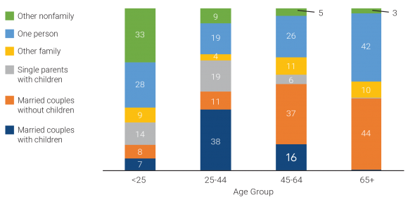
Percent Distribution of U.S. Household Types by Age of Householder, 2017

Notes: Percentages may not sum to 100 due to rounding. Among householders ages 65 and older, 0.4 percent headed married-couple households with children and 0.1 percent headed single-parent households with children.
Sources: U.S. Census Bureau, 2017 American Community Survey Public Use Microdata Sample (PUMS).


In contrast, the split between family and nonfamily households is reversed among householders ages 25 to 44—only 28 percent headed nonfamily households and 72 percent headed family households. While only one-fifth of households headed by an adult under age 25 included children, almost three-fifths (56 percent) of householders ages 25 to 44 headed families with children—both married-couple families (38 percent) and single-parent families (19 percent). Only 11 percent headed married-couple families without children. About one-fifth (19 percent) of householders in this age group lived alone in 2017, but less than one in 10 (9 percent) headed 2+-person nonfamily households—down from 33 percent among householders under age 25.

More than a third of householders ages 45 to 64 (37 percent) were empty nesters, heading married-couple households without children. Only about one-fifth (21 percent) of householders ages 45 to 64 headed families with children—16 percent were married-couple families and only 6 percent were single-parent families. However, a relatively high share of householders ages 45 to 64 were heading other family households (11 percent) and one-person households (26 percent).

Eight in 10 householders ages 65 and older were either heading married-couple families without children (44 percent) or living alone (42 percent). Only 10 percent of householders in this oldest age group headed other family households and only 3 percent headed other nonfamily households.

What’s Driving Changes in Household Composition?

Beginning in the 1960s—and accelerating over the last two decades—changes in marriage, cohabitation, and childbearing have played a key role in transforming household composition in the United States. More recently, population aging and shifts in the age distribution of householders are also contributing to these changes in composition.

Young Adults Continue to Delay Marriage and Childbearing

Delays in marriage and childbearing and increases in cohabitation among young adults have contributed to the decline in the share of family households—particularly married couples with children—and the steep rise in the share of nonfamily households. The median age at first marriage reached a new high in 2017—29.5 for men and 27.1 for women—and cohabitation rates have continued to increase.6 In 2011-2013, 65 percent of women ages 19 to 44 reported having had a cohabiting relationship, up from 33 percent in 1987.7

Birth rates among women under age 30 have continued to decline since 2010, although the rates for women ages 30 to 34 increased through 2016 before decreasing from 2016 to 2017.8 The share of births to women under age 40 that occurred outside of marriage increased from about 21 percent in 1980-1984 to 43 percent in 2009-2013; about 60 percent of the nonmarital births in 2009-2013 were to cohabiting couples—up from only 28 percent in 1980-1984.9

Between 2000 and 2010, the increase in cohabiting couples with children contributed to growth in the shares of both single-parent families and other nonfamily households due to the ways the Census Bureau classifies such couples by household type. However, between 2010 and 2017, the share of other nonfamily households stayed constant, and the share of single-parent families declined slightly from 10 percent to 9 percent. This decrease may be due to the drop from 18 percent to 14 percent in the share of householders under age 25 who were heading single-parent families. While declining birth rates among young women are partly responsible, this decline could also be related to more young couples with children living with their parents rather than in their own households. This explanation is supported by evidence of an increase in the number of multigenerational households, which rose from 4.4 million in 2010 to 4.6 million in 2017.

A Growing Share of Householders Are Ages 65 and Older

As fertility rates have fallen and baby boomers have aged, the distribution of the adult population ages 18 and older in the United States has shifted to older age groups. Between 2010 and 2017, the share of adults ages 45 to 64 declined from 35 percent to 33 percent, while the share ages 65 and older increased from 17 percent to 20 percent. About 22 percent of the adult population is projected to be age 65 or older by 2020.

These shifts in the age distribution of the adult population have been accompanied by changes in the age distribution of householders. Between 2010 and 2017, the shares of householders under age 25, ages 25 to 44, and ages 45 to 64 all declined by 1 or 2 percentage points, while the share of householders ages 65 and older increased by nearly 4 percentage points. This increase in the share of older householders is contributing to growth in the shares of both married-couple households without children and one-person households. These trends are likely to continue as more baby boomers enter older age groups in the coming decades.

Fewer Young Adults Are Forming New Households

Young adults forming new, independent households—alone, with a spouse or partner, or with unrelated roommates—has historically been an important factor in the overall household growth rate. Between 2010 and 2017, the young adult population (ages 18 to 34) increased by 4.2 million, accounting for nearly a quarter of the growth in the adult population (ages 18 and older).10 Yet, the household growth rate slowed to only 3 percent during this period—much lower than the 11 percent growth rate between 2000 and 2010. While the living arrangements of adults ages 35 to 64 have remained stable, recent changes in young adults’ living arrangements help explain the decline.

The share of young adults ages 18 to 34 who have formed an independent household has declined since 2010, while the share living with their parents has increased sharply. In 2010, less than one-third (32 percent) of young adults ages 18 to 34 were living with their parent(s), but this share jumped to 35 percent by 2017. The increase was sharpest among 25- to 29-year-olds, rising from 21 percent in 2010 to 26 percent in 2017 (see Figure 2). The share of 30- to 34-year-olds living with their parent(s) also increased by 4 percentage points across this period. In contrast, the share of young adults living in a married-couple family declined for all age groups between 2010 and 2017, with the largest drop among those ages 25 to 29.

FIGURE 2. Share of Young Adults Living With Their Parents Increases, While Share Living With a Spouse Declines

article4-fig2@4x

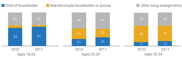
Selected Living Arrangements of Young Adults Ages 18 to 34 (%), 2010 to 2017

Notes: “Other living arrangements” include householders living alone, with an unmarried partner, with other relatives, or with nonrelatives. Percentages may not sum to 100 due to rounding.
Source: U.S. Census Bureau, 2010 and 2017 American Community Survey PUMS.


The Great Recession and the slow economic recovery, high student debt loads, and high relative housing costs have all likely contributed to the declining shares of young adults forming or maintaining independent households since 2010. Whether these patterns persist into 2020 and beyond is an open question. If the job market and earnings continue to improve, the ability of young adults to form new households may increase. If housing costs continue to rise, however, the resulting economic burden on young adults may counteract any improvements in employment and earnings and dampen household growth rates in the future.


This article is excerpted from Mark Mather et al., “What the 2020 Census Will Tell Us About a Changing America,” Population Bulletin 74, no. 1 (2019).


References

  1. Frank Hobbs and Nicole Stoops, Demographic Trends in the 20th Century (2002), Figure 5-3; and U.S. Census Bureau, 2010 Census Summary File 1.
  2. Hobbs and Stoops, Demographic Trends in the 20th Century, Figure 5-2.
  3. U.S. Census Bureau, 2010 Census Summary File 1.
  4. U.S. Census Bureau, 2017 American Community Survey.
  5. Hobbs and Stoops, Demographic Trends in the 20th Century, Table 5.
  6. U.S. Census Bureau, “Table MS-2. Estimated Median Age at First Marriage, by Sex: 1890 to the Present,” www.census.gov/data/tables/time-series/demo/families/marital.html.
  7. Wendy D. Manning and Bart Sykes, Twenty-Five Years of Change in Cohabitation in the United States, 1987-2013, FP-15-01 (Bowling Green, OH: National Center for Family and Marriage Research, 2015); Larry L. Bumpass and James A. Sweet, “National Estimates of Cohabitation,” Demography 26, no. 4 (1989): 615-25.
  8. Joyce A. Martin et al., “Births: Final Data for 2017,” National Vital Statistics Reports 67, no 8 (2018).
  9. Wendy D. Manning, Susan L. Brown, and Bart Sykes, Trends in Birth to Single and Cohabiting Mothers, 1980-2013, FP-15-03 (Bowling Green, OH: National Center for Family and Marriage Research, 2015); and Joyce A. Martin et al., “Births: Final Data for 2017.”
  10. U.S. Census Bureau, Vintage 2017 Population Estimates.
Women walking toward the camera.

Eliminating Smoking and Obesity Could Shrink U.S. Health Disparities, But Where People Live Matters Too

Smoking and obesity are the two leading causes of preventable death, disability, and chronic disease in the United States. New research shows that eliminating them could go a long way in reducing racial health gaps. But location also plays a key role in health disparities, with neighborhood setting and state-level policies shaping residents’ health, this new study and another suggest.1

“We know that, compared to white peers, black men and women enjoy fewer years of life expectancy and healthy life expectancy, which is the number of years individuals can expect to live without disability. Meanwhile, immigrant- and U.S.-born Hispanics live longer than U.S.-born whites, despite their ethnic minority and lower socioeconomic status,” says Michelle Frisco of Penn State University, who conducted the first study with her Penn State colleague Jennifer Van Hook and Robert Hummer of the University of North Carolina, Chapel Hill. Their research was supported by the Eunice Kennedy Shriver National Institute of Child Health and Human Development (NICHD).

The researchers wanted to explore how obesity and smoking contributed to these differences because both health problems are concentrated in some groups in ways that are likely to produce health disparities. For example, white men and women smoke more than Hispanic immigrants, and black women are more likely to be obese and have a tougher time quitting smoking than white women.

Eliminating Smoking and Obesity Would Reduce the Black-White Health Gap

The research team analyzed data on health and mortality from almost 20,000 U.S.-born white, black, Hispanic, and foreign-born Hispanic men and women from the National Health and Nutrition Examination Survey. They focused on life expectancy and years spent disability-free for each racial or ethnic group. They then simulated how many years each group could expect to live overall and disability-free if no one ever smoked or was obese. Their findings showed some striking reductions in group differences.

“The actual disparity in the life expectancy between white and black women in the U.S. is approximately two years,” Frisco reports. “When we simulated the elimination of smoking and obesity, that gap was reduced to three months. Nearly every significant group difference was reduced to the point that gaps between groups were no longer statistically significant.”

There was one exception: Foreign-born Hispanic men and women retained their nearly three-year life-expectancy advantage over white peers even when the simulation eliminated both obesity and smoking.

“Hispanic immigrants typically have a longer life expectancy than whites to begin with. Eliminating obesity and smoking did not change this,” says Frisco. Not only do Hispanic immigrants smoke less than their U.S.-born peers, they are more likely to eat diets healthier than the typical American diet and live in tight-knit communities with widespread social support. They are also less likely to have substance abuse disorders, according to the researchers. In addition, they report that Hispanics who migrate to the United States tend to be healthier than their counterparts who remain in their country of origin.

Not Just Individual Behavior—Neighborhood Setting Shapes Health

The findings suggest that interventions aimed at preventing obesity and weight gain, reducing smoking, and increasing smoking cessation could be more effective if they’re tailored to specific populations. However, the researchers noted that these programs shouldn’t blame the victim by focusing only on individual behavior.

“We know that the places where people live influence smoking and obesity. For example, segregation leads U.S. black men and women to have elevated risks of long-term smoking and obesity in part because of the ways that tobacco companies disproportionately target minority neighborhoods, as do fast food restaurants and corporations who sell soda. These and other forms of structural racism must be addressed if we want to ensure greater health equity in the U.S.,” Frisco says.

The Disproportionate Health Consequences of State Policies

Some states invest more heavily in the health and well-being of their people, and these investments have “disproportionate consequences” for people with low education and income levels, Mark Hayward of the University of Texas at Austin, Jennifer Montez of Syracuse University, and Anna Zajacova of Western University show in the second study.

American adults with less education tend to report more chronic diseases and disabilities, and die sooner than those with more education, and these disparities have widened in recent decades, according to Hayward.

While more-educated people usually have higher incomes and less physically demanding jobs than less-educated people, the dynamics are more complicated than that, he explains. Blaming lifestyle differences between the two groups neglects the economic and social contexts where people live, he says.


A college education acts as a ‘personal firewall,’ protecting a person wherever they live.


The research team analyzed state-level health data on U.S-born adults ages 45 to 89 in two nationally representative data sets—the National Longitudinal Mortality Study and the American Community Survey. They focused on seven health measures including various functional difficulties, and problems with mobility, vision, hearing, and cognition, as well as overall self-reported health.

They found that the health gap between more- and less-educated people varies widely among states. The size of that gap is mainly related to the health levels of adults with less education.

A college education acts as a “personal firewall,” protecting a person wherever they live, Hayward suggests. “Well-educated persons have better access and support for healthy lifestyles and care, good jobs and rewards, and valuable networks and relationships, and they have sophisticated cognitive skills and a greater sense of control and human agency,” he says. By contrast, less-educated people are more vulnerable to differences in state policies and programs “precisely because they have fewer personal resources and are exposed to greater risks.”

The researchers point to Massachusetts and Mississippi to illustrate the wide differences in state-related policies affecting health. Unlike Massachusetts, Mississippi does not supplement the Earned Income Tax Credit that benefits working poor families, did not expand state Medicaid coverage following the 2010 Affordable Care Act, and has limited cigarette sales taxes.

Policies among the 50 U.S. states began to diverge in the 1970s with devolution—national policy changes that allowed states to opt out of federal programs and gave them more discretion over the services they offered.

Cigarette Taxes Influence Who Smokes

Hayward and colleagues explore excise taxes on cigarettes as an example of state-level policy differences that drive health disparities. Previous research has shown that tobacco control policies such as cigarette excise taxes shape smoking behavior.2

Hayward and colleagues find that smoking prevalence differs widely by state among less-educated people but is similar among those with higher levels of education. They show that state cigarette tax levels influence the prevalence of smoking among less-educated people but have a limited effect on their more-educated peers. Less-educated people tend to smoke less if cigarette taxes are high, while more-educated people have more resources and experience other incentives and disincentives to smoking, they suggest.

The five states with the largest increases in cigarette excise taxes between 1990 and 2014 saw smoking prevalence differences between less- and more-educated adults shrink by two-thirds—from an 11.2 percentage-point gap to a 3.8 percentage-point gap. But the gap nearly doubled in the five states with the smallest increases in state cigarette excise taxes, from a difference of 8.4 percentage points to 16.1 percentage points.

How Can We Close the Health Gap?

The adverse health effects of low education levels are much less evident in states with strong social safety nets and policies that encourage investments in residents’ health and well-being, Hayward reports. “These types of state policies and contextual factors can compensate for the effects of low education on health.”

When social safety nets are weak and investment in the well-being of their populations is low, states can exacerbate the health effects of low education, he suggests.

“States have become a major institutional force affecting incentives and capacities of residents to create healthy lives,” he says. This study on cigarette taxes and health is part of a growing body of research on the impact of state policy differences on health. Earlier studies by Hayward and colleagues show that state policies contribute to state-level differences in premature deaths and disability, particularly among less-educated women.3


This article was produced under a grant from the Eunice Kennedy Shriver National Institute of Child Health and Human Development (NICHD). The work of researchers from the following NICHD-funded population dynamics research centers was highlighted in this article: Penn State University, University of North Carolina at Chapel Hill, and University of Texas at Austin.


References

  1. Michelle L. Frisco, Jennifer Van Hook, and Robert A. Hummer, “Would the Elimination of Obesity and Smoking Reduce U.S. Racial/Ethnic/Nativity Disparities in Total and Healthy Life Expectancy?” SSM Population Health 7, no. 1 (2019); and Jennifer Karas Montez, Mark D. Hayward, and Anna Zajacova, “Educational Disparities in Adult Health: U.S. States as Institutional Actors on the Association,” Socius 5, no. 1 (2019): 1-14.
  2. Chloe E. Bird and Patricia P. Rieker, Gender and Health: The Effects of Constrained Choices and Social Policies (New York, Cambridge University Press: 2018).
  3. Mark D. Hayward, Robert A. Hummer, and Isaac Sasson, “Trends and Group Differences in the Association Between Educational Attainment and U.S. Adult Mortality: Implications for Understanding Education’s Causal Influence,” Social Science and Medicine 127, no. 1 (2015): 8-18; Jennifer Karas Montez, Anna Zajacova, and Mark D. Hayward, “Explaining Inequalities in Women’s Mortality Between U.S. States,” SSMPopulation Health 2, no. 1 (2016): 561-71; Jennifer Karas Montez, Anna Zajacova, and Mark D. Hayward, “Disparities in Disability by Educational Attainment Across U.S. States,” American Journal of Public Health 107, no. 1 (2017): 1101-8; Jennifer Karas Montez, Mark D. Hayward, and Douglas A. Wolf, “Do U.S. States’ Socioeconomic and Policy Contexts Shape Adult Disability?” Social Science and Medicine 178, no. 1 (2017): 115-26; and Jennifer Karas Montez, “Deregulation, Devolution, and State Preemption Laws’ Impact on U.S. Mortality Trends,” American Journal of Public Health 107, no. 1 (2017): 1749-50.